Bintang-bintang-Sebuah Pengantar
Bintang-bintang adalah serupa sebagaimana matahari kita, namun banyak aneka ragam variasi dari bintang-bintang ini. Satu hal menyangkut bintang adalah, semua bintang lahir dari fusi nuklir yang terjadi di inti mereka.
Hampir setiap titik-titik cahaya yang berkelip di angkasa yang kita lihat merupakan bintang-bintang. Semua bintang tersebut berada di dalam Galaksi Bima Sakti kita (
Milky Way
Galaxy). Sangat jarang bintang tersebut menyendiri berada di ruang antar Galaksi, dan normalnya bintang-bintang senantiasa berada dalam Galaksi (
galaxies).
Ada dua grup bintang-bintang:
- Bintang populasi II - bintang tua, kurang mengandung logam
- Bintang populasi I - bintang muda, bintang-bintang yang kaya dengan logam
- Bintang normal ( Normal stars )- seperti matahari kita (Sun) - Bintang seperti ini akhir hidupnya menjadi Nebula Planet atau Bintang Katai Putih
- Bintang besar (Large stars) di mana akhir hidupnya adalah menjadi sebuah supernova atau berakhir menjadi Bintang Neutron dan Lubang Hitam (Black Hole)
- Awan debu membentuk bintang deret utama yang akan menyala selama 10 milyar tahun
- Kehidupan bintang berakhir di deret utama untuk kemudian menjadi Raksasa Merah (seukuran orbit bumi) dan menyala selama 100 juta tahun
- Lapisan bakal bintang menjadi Nebula Planet yang berlangsung selama 100.000 tahun
- Hanya inti bintang yang tetap sebagai bintang Katai Putih
- Awan debu membentuk sebuah bintang besar yang tetap bersinar di deret utama selama 50 juta tahun.
- Bintang tetap berada di masa hidup deret utama sebelum berakhir menjadi maha raksasa merah (kira-kira seukuran orbit planet Mars) dan bersinar dalam keadaan ini selama satu juta tahun.
- Core collapse can occur anytime after the million year Red Supergiant phase, and can go supernova
- All that is left is a supernova remnant (a wispy looking nebula) and a compact object - Neutron Star or Black Hole
- Open Clusters - a group of "new" stars in a group with a few hundred members
- Globular Clusters - a group of "old" stars in a group with a few thousand members
- Galaxies
Open clusters and globular clusters will be discussed in greater detail in their own sections.
Of course, a star does not have to be in an open or globular cluster but almost always a star will be a part of a galaxy.
Back to Top
But how does the life of a star begin?
The most abundant material in the Universe is Hydrogen. Clumped together in cold clouds, hydrogen atoms can join together to form molecular hydrogen. This only occurs at extremely low temperatures.
 |
These molecular clouds are very difficult to detect because no emission occurs. Much of the interstellar reddening (where a star or galaxy appears more red) occurs because of these molecular clouds. The image on the left is Barnard 68, a dark nebula. This is what a molecular cloud "looks" like. Notice the stars are barely visible behind this cloud. However, it is possible to view what's behind the cloud using an infrared filter. |
- Jeans Mass
- Jeans Length
Jeans length basically states
that a molecular cloud of a particular size can
become unstable and begin collapse.
The Radius in the above equation
is Jeans Length, the minimum radius of the cloud
before self-gravitation occurs.
 |
The table on the left give some examples of the density of molecular clouds and the resulting size of the cloud. Within a molecular cloud, the distribution of debris is not always even. Fragmentation is suspected to occur in clouds exceeding |
So what can cause a molecular cloud to collapse?
- Nearby stars that have ended their live in a supernova can send a shockwave stimulating collapse
- Density waves within a galaxy propagate through the spiral structures that can stimulate collapse
- Galaxy collisions can create huge gravitational forces to act of nearby clouds
- A nearby Wolf-Rayet star can stimulate collapse
- Sequential stellar formation - nearby stars forming close enough that their initial fusion can stimulate collapse
| As the molecular contracts under its own gravity, conservation of momentum forces the cloud to take on a disk shape, and it begins to spin. The very center of the cloud remains circular while the outlying gas forms a disk. Material from this disk is ejected perpendicular to to the disk as seen on the right. |  (Image credit: Brooks/Cole Thomson Learning) |

It is important to know that
there is a limit to stellar formation. The
proto-star must fall within a:
-
lower limit mass of 0.8 Solar masses
-
an upper limit mass of 100 Solar Masses
A proto-star that is less than
0.8 Solar masses becomes a Brown Dwarf and a
proto-star that exceeds 100 Solar masses becomes
a Wolf-Rayet star - a very unstable star that
cannot hold on to its outer layers.
As the Hydrogen
atoms at the
core of the proto-star are forced together by
heat and pressure, the Coulomb Barrier is
reached.
(Image credit: Brooks/Cole Thomson Learning)
The above image demonstrates
that as the radius, r, or the space between
protons is limited, a
strong attractive force
occurs.
(Image credit: Brooks/Cole Thomson Learning)
The Proton-Proton Chain begins
with the fusing of hydrogen
atoms into helium
atoms - plus some gamma rays,
neutrinos and
photons.
Notice the times in the image
above. It can take 1,000,000,000 years for the
hydrogen
atoms to exceed the Coulomb Barrier.
So what is the equation that
demonstrates the energy produced by this
reaction?
A T-Tauri star is a proto-star
that has begun its fusion burning stage - with a
bang and a shock wave that blows away any nearby
debris close to the star.
I know this may seem like an
overwhelming amount of information for an
introduction, almost as complicated as trying to learn and understand the new system of POS software that came with the online store
if there hadn't been some assistance available in learning the software
along the way, but these pages are meant to aid you along as well. The following pages will revisit some of this material providing some insight with some real-world examples.
Stellar Astrophysics - the study
of the stellar process - is not an easy subject,
but hopefully this information will bring you
one step closer to fully understanding the
processes of not only our
Sun, but all of the
stars in the
night sky.
While stars are just point sources far from Earth, there is still much we can learn. For example, if the star is relatively close to us, we can determine its distance using stellar parallax:
(Image Credit: Pearson Education, Addison Wesley)
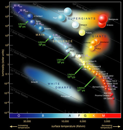
In addition, notice the x-axis of the H-R diagram. This is the spectral class - the result of the Harvard team.

(Image Credit: Pearson Education, Addison Wesley)
The famous pneumonic helps astronomers remember
this sequence: Oh Be A Fine
Girl (or Guy) and Kiss Me.
Who says scientists don't have a sense of humor?
One final interesting formula: a quick and dirty correlation between a stars luminosity and magnitude is:
 All that is left is to determine the mass of a
star. We now know that bright stars are very large
and dim stars are small, but without an accurate
measure of mass, we can only speculate. This is
where binary stars come into play.
All that is left is to determine the mass of a
star. We now know that bright stars are very large
and dim stars are small, but without an accurate
measure of mass, we can only speculate. This is
where binary stars come into play.
Back to Top
A binary star is a multiple star system bound by mutual gravitation. Both stars will revolve about a common point. By using Keplerian math, we can determine the mass by studying this movement. If we know the spectral class of the stars in question, we can assign standardized values (like the H-R diagram) that will give is the mass of all stars.
There are four main classes of binary stars:
(Image credit: Brooks/Cole Thomson Learning)
In order to find the mass of a visual binary:
(Image credit: Brooks/Cole Thomson Learning)
m in this case is mass and P is the period of the
orbit.
A spectroscopic binary star is one that is not seen visually, but long term observation records a shift in the stars spectrum:
(Image credit: Brooks/Cole Thomson Learning)
Sometimes if the orbit of the binary star is
facing us, we may not be able to see
spectroscopic
changes, but we will see
brightness changes. Long
term observation will reveal periodic changes in
overall
brightness:
(Image credit: Brooks/Cole Thomson Learning)
Stars - Stellar Classifications
A star is classified by
luminosity and color.
luminosity is measure in
magnitudes and color is
measured by temperature. Edward Pickering and Willimina Fleming and a group of women (one of these
women, Henrietta Leavitt, discovered the
Cepheid
variable star - important in distance measurements)
cataloged thousands of stars according to spectra.
While all the this number data was fine, it was two
astronomers (working separately) that discovered a
correlation to a stars spectra and
brightness. Ejnar
Hertzsprung and Henry Norris Russell created a plot
of the stars and created what is now called the
Hertzsprung-Russell diagram. We will look at this
diagram later.
While our observations can
determine
luminosity and spectral classes, close
observation and study of
binary stars can also yield mass.While stars are just point sources far from Earth, there is still much we can learn. For example, if the star is relatively close to us, we can determine its distance using stellar parallax:
By measuring the shift angle seen
from
Earth, we can determine distance. In case you
don't know what
parallax is, hold a pen or pencil
arms length from your face and close one eye at a
time while looking at something far away. The
shifting of the pen is the
parallax.
We can also determine the
brightness of a star (as well as its
luminosity) if we know its
distance. We can use the Inverse Square Law:
However, notice that we need to know
the
luminosity of the star to determine
brightness.
We can determine the
luminosity of the star using
this formula:
but without knowing
brightness, it
seems we cannot determine
luminosity. This is where
our
Sun comes in. We have the benefit of a
frame of reference when comparing to other stars.
With the known values in place, its
just a matter of some
algebra.
Another classification for stars is
magnitude - how bright does the star appear to us on
Earth. There are two versions of
magnitude:
The
magnitude scale is graded by
numbers: 0 being bright, 6 being dim. Some values of
comparison:
-
Our Sun - -26.7 (that's a negative)
-
Sirius - -1.4
-
Naked eye limit - +6.0
-
Binocular limit - +10.0
-
Pluto - +15.1
-
The Hubble Space Telescope limit - +30.0
The
magnitude scale works out to be
logarithmic, and the difference between each value
is 2.512. That is
magnitude 1 is 2.512 times
brighter than
magnitude 2 and
magnitude 5 is 2.512 *
2.512 * 2.512 times dimmer that
magnitude 2.
By knowing the distance and apparent
magnitude to a star, we can learn the absolute
magnitude. Also, if we happen to know the absolute
magnitude, we can determine distance. The result of
this is the distance modulus:
or:
By using filters (blue, green, red)
and measuring the
brightness of a star in the
different filters, we can determine the color index
of a star (and recall from the physics section that
color and temperature go hand in hand):
If the B-V value is 1, the star is
white. If the B-V index is less than 1, the star is
more blue and if the B-V index is more than 1, the
star is more red.
All of these tools led to a
correlation: a stars size relates to how bright it
and how hot it is.
It is this correlation that helped
to create the Hertzsprung-Russell (or H-R) diagram:
(Image Credit: Pearson Education, Addison Wesley)
Going back to
luminosity, there are
six classes of
luminosity:
- Ia - Bright Supergiant Stars (example: Deneb)
- Ib - Supergiants (example: Antares)
- II - Bright Giants (example: Canopus)
- III - Giants (example: Capella)
- IV - Subgiants (example: Beta Cru)
- V - Main Sequence (example: Vega)
In addition, notice the x-axis of the H-R diagram. This is the spectral class - the result of the Harvard team.
- O - O type stars are the brightest and the live the shortest
- B - B type stars are blue white and also burn bright, but not as bright as the O type
- A - A type stars are less bright, a little larger than our Sun, but still burn hotter
- F - Brighter than our Sun and a little hotter
- G - Our Sun is a G type star
- K - dimmer that our Sun, will burn longer because temperature is lower
- M - the dimmest stars, will burn for a long time
(Image Credit: Pearson Education, Addison Wesley)
One final interesting formula: a quick and dirty correlation between a stars luminosity and magnitude is:
Back to Top
A binary star is a multiple star system bound by mutual gravitation. Both stars will revolve about a common point. By using Keplerian math, we can determine the mass by studying this movement. If we know the spectral class of the stars in question, we can assign standardized values (like the H-R diagram) that will give is the mass of all stars.
There are four main classes of binary stars:
- Visual binary stars - stars that we see on Earth as being binary
- Spectroscopic binaries - binary stars that are only seen using spectroscopy
- Eclipsing binaries - binary stars at our line of sight
- Accreting binaries - close pairs that "feed" off each other
(Image credit: Brooks/Cole Thomson Learning)
(Image credit: Brooks/Cole Thomson Learning)
A spectroscopic binary star is one that is not seen visually, but long term observation records a shift in the stars spectrum:
(Image credit: Brooks/Cole Thomson Learning)
(Image credit: Brooks/Cole Thomson Learning)
This same technique is used for the
detection of
exoplanets.
The final class of binary star is the accreting
binary. If the pair of stars are close enough, the
atmosphere of one star can pour onto another. The
point of no return in this case is the outer
Lagrange point (not seen in the image). If material
breaches the outer Lagrange point and contacts the
inner Lagrange point, material will begin to flow
onto another (that is what I mean by the point of no
return).
(Image credit: Brooks/Cole Thomson Learning)
(Image credit: Brooks/Cole Thomson Learning)
A common companion star to an accreting binary
system is a neutron star or a white dwarf - both
covered in
stellar evolution.
Some final
bits: binary star system are actually quite common -
Sir William Herschel discovered 10,000 binary star
systems. In addition, binary stars are really part
of multi-star systems. Many stars have more than one
companion. A triple star system is also common.
To sum up, here is a nice chart I found that
demonstrates the process of stellar classification:
Stars - Stellar Populations
Population II stars were believed to have formed first. These stars occupy the globular clusters that reside in the halo of the galaxy. However, it should be noted that the search is on for Population III stars. Astronomers suggest that the very first stars to ever form in the universe were Population III - that only burned hydrogen and helium only. The suggested comes from the determination that most Population II stars do have some heavy elements.
Some characteristics between a Population II star versus a Population I star is:
Astronomers believe this has to do with the opacity of the stellar atmosphere. More metals mean a more opaque atmosphere in a Population I means less energy escapes (when compared to Population II stars anyway).
So how does a Population I star contain metal when a Population II star does not?
We will cover this in stellar evolution, but much of the heavy elements in our Universe today is created when a giant star end its life in a supernova. The intense heat for this creates in the upper atmosphere of stars much of the elements we know - like iron, gold, even fluoride (yes, the same stuff in your toothpaste).
These elements disperse themselves to nearby molecular clouds. When that cloud undergoes contraction and give birth to a new star, the end result is a Population I star - one that is now metal rich.
One consequence of a metal rich star is that they are likely to contain a system of planets!
Stars - Stellar Populations
Stars can be grouped by various populations. The most obvious being star cluster: globular clusters and open clusters.
More specifically stars can be divided by main population based on Metallicity.- Population I stars - new stars that contain numerous heavy metals in their atmosphere
- Population II stars - old stars that contain little heavy metals in their atmosphere
Population II stars were believed to have formed first. These stars occupy the globular clusters that reside in the halo of the galaxy. However, it should be noted that the search is on for Population III stars. Astronomers suggest that the very first stars to ever form in the universe were Population III - that only burned hydrogen and helium only. The suggested comes from the determination that most Population II stars do have some heavy elements.
Some characteristics between a Population II star versus a Population I star is:
- Population II stars burn hotter
- Population II stars burn faster
Astronomers believe this has to do with the opacity of the stellar atmosphere. More metals mean a more opaque atmosphere in a Population I means less energy escapes (when compared to Population II stars anyway).
So how does a Population I star contain metal when a Population II star does not?
We will cover this in stellar evolution, but much of the heavy elements in our Universe today is created when a giant star end its life in a supernova. The intense heat for this creates in the upper atmosphere of stars much of the elements we know - like iron, gold, even fluoride (yes, the same stuff in your toothpaste).
These elements disperse themselves to nearby molecular clouds. When that cloud undergoes contraction and give birth to a new star, the end result is a Population I star - one that is now metal rich.
One consequence of a metal rich star is that they are likely to contain a system of planets!
Tidak ada komentar:
Posting Komentar